Click to learn more about author Steve Miller.
I ran across an R forecasting package recently, prophet, I hadn’t seen before. This isn’t surprising given the flood of new libraries now emerging in the R ecosystem.
Developed by two Facebook Data Scientists, what struck me most about prophet was the alignment of its sweet spot problem domain with consulting work I’d done a few years ago in digital marketing for a large media company. With that engagement, the challenge was forecasting hundreds of daily time series, each with several years of historical data. Patterns manifested included trend and multiple seasons. Predictions were desired over an entire year, and models were to be updated weekly with the latest data.
I started the work with a pretty standard bag of statistical forecasting tricks, including moving averages, seasonal and trend decomposition, exponential smoothing such as Holt Winters, ARIMA, and even a few econometric alternatives. Alas, after none of these attempts even closely nailed it, I turned to traditional regression and more modern machine learning approaches though, given autocorrelation of disturbances, these are generally considered anathema for forecasting by statistical purists. I was getting desperate, however. A statistical consolation was that I was just interested in the quality of predictions, not overall model purity.
So when I read that: “Prophet is a procedure for forecasting time series data. It is based on an additive model where non-linear trends are fit with yearly and weekly seasonality, plus holidays. It works best with daily periodicity data with at least one year of historical data. Prophet is robust to missing data, shifts in the trend, and large outliers.”, I just had to test it out. Could this be what I needed years ago?
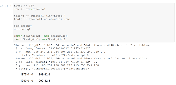
A data set I’d used to prep for the digital media engagement was daily births in Quebec from 1977-1991. Quebec represents counts of 14 years of daily newborn deliveries in the Canadian province. It served nicely for simulating my digital marketing challenges and I figured it could now help me put prophet through its paces as well.
The remainder of this post examines the results of several modeling exercises in R against the Quebec data divided into train with 13 years and test with one. prophet is compared against a basic linear model (lm), a general additive model (gam), and random forests (randomForest).
At the start, set a few options, load some libraries, and change the working directory.

Read the Quebec births file, building a data.table with variable names “ds” and “y” representing the date and birth counts to accommodate prophet. Create train and test data.tables — train with the first 13 years of daily data, test with the 14th year.

Define two little functions to compute root mean square error (rmse) and mean absolute percentage error (mape) of actual vs predicted a la forecast for evaluating forecast model performance. Lower is better.

Now start fitting basic lm linear models. The first regresses dailybirths (y) on a cubic spline of the integer date (ds) to capture trend. Compute the rmse and mape against the training and test data. Not surprisingly, the stats for train are better than for test.
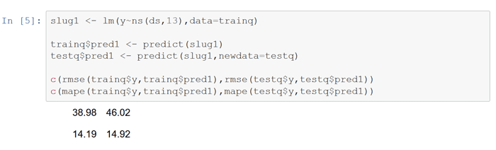
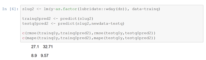
Next run a model of dailybirths on a day of the week factor to capture intra-week seasonality. This model appears to do better than the first on the preformance metrics, indicating significant day of the week seasonality.
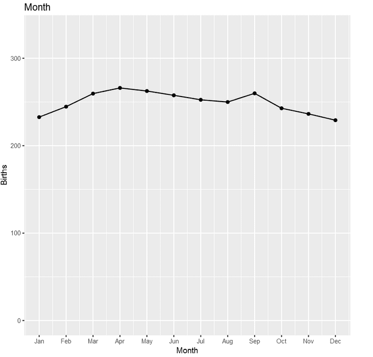
The third model creates a factor based on month to handle monthly seasons. This seasonality doesn’t appear to be as strong as day of the week.

Finally, run an lm model that includes all three variables above. Note the predictively sanguine lower rmse and mape.

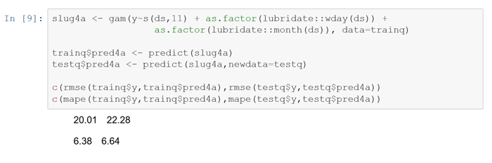
Now run a similar 3 variable general additive model with the gam package. Not surprisingly, the rmse and mape for both train and test are comparable to the final lm model.
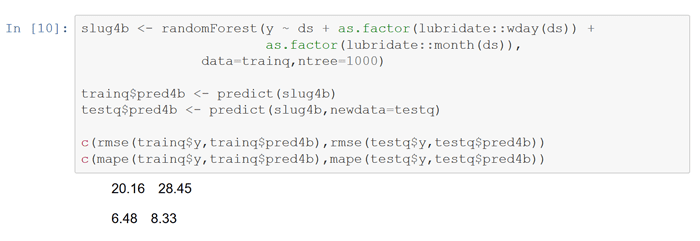
Fit a randomForest ML model using similar trend and seasonality attributes. Note the larger disparity between train and test performance, indicating overfit to the train data.
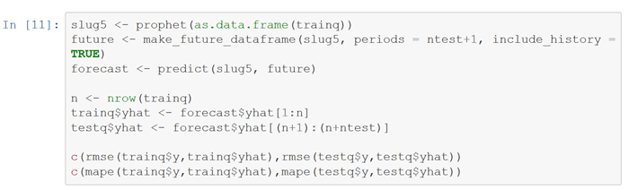
Finally partition the data into train and test suitable for prophet and fit its model

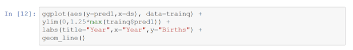
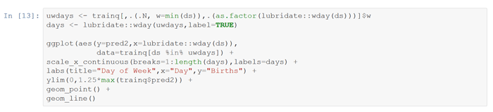
At this point, let’s take a look at predictions from the various lm models fitted above – first trend, then day of the week, and finally month.


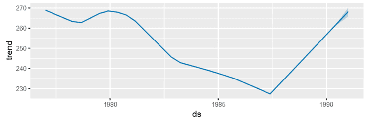
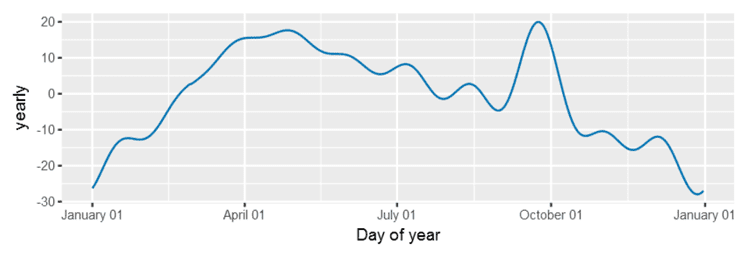
Next graph the components of the prophet model, which look a lot like the charts above – except that prophet uses day of the year in contrast to month.
![]()

Finally, compare the 3-attribute lm model, the gam model, the prophet model, and the random forest model using the test data. In each panel, the grey denotes actual values while the colors represent model predictions. lm, gam, and prophet perform similarly, while random forest lags.


With this particular data, the test predictions of the prophet, lm and gam models are quite similar – and superior to randomForest. This is just one evaluation, but prophet performing as well as the parameterized models here is very encouraging. If prophet’s flexible enough to handle other challenges it could indeed live up to the “forecasting at scale” claim. prophet, where were you when I was in need?